With the ever increasing number of single cell transcriptomics data sets available, people are wanting to do combined analyses more and more frequently. Of course, the first thing that happens when people do this is that data from different samples, labs, and experiments don’t “mix well”. The identification of poor mixing is mostly done on the basis of cell annotation and inspection of dimension reduction plots made with UMAP and/or tSNE. The response is usually to apply some, kind, of batch correction.

The most information rich scRNA-seq experiments are still fresh tissue experiments, which require fresh tissue. This requirement prevents balanced experimental design, as samples most be processed sequentially as and when tissue becomes available. Consequentially, this issue of batch effects arises even in contained experiments performed with the same technique in the same lab.

In the first of a series of posts, I will argue that as a field we are over-diagnosing and over-correcting for batch effects. This is not to say that batch correction should never be used. I have contributed to a single cell batch correction method myself. But I think in rushing to correct everything that looks like a batch effect we are masking interesting biology.

Diagnosis of batch effects

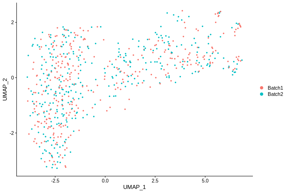
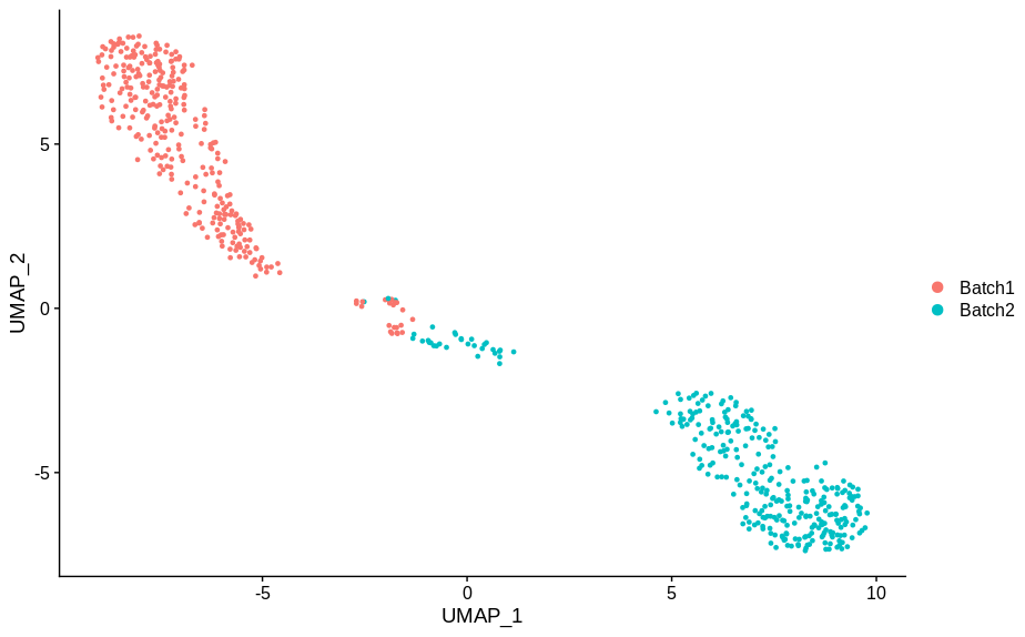
Let’s start by looking at a plot. Let’s say that we have two samples, and have run the 10X 3’ gene assay on the same tissue from both of them.

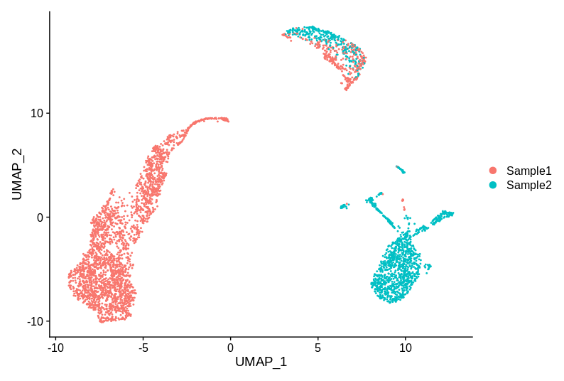
This example is entirely made up (although uses real data), but I have seen plots that have the same key properties. So, does this data have batch effects that need correcting? The cluster of cells at the top is reasonably well mixed, but the groups on the left and right are specific to each sample. So bring out the batch correction? Or not?

My question is not really a practical one of should I apply batch correction and if so should I use method X, Y, or Z. I am asking something more fundamental. Is there a batch effect here that I need to worry about and employ some tools to help me correct for? Some might argue that any sensible batch correction method will do nothing, or very little when no batch effect is present. But no method is perfect and we should not do things to the data that we don’t have to.

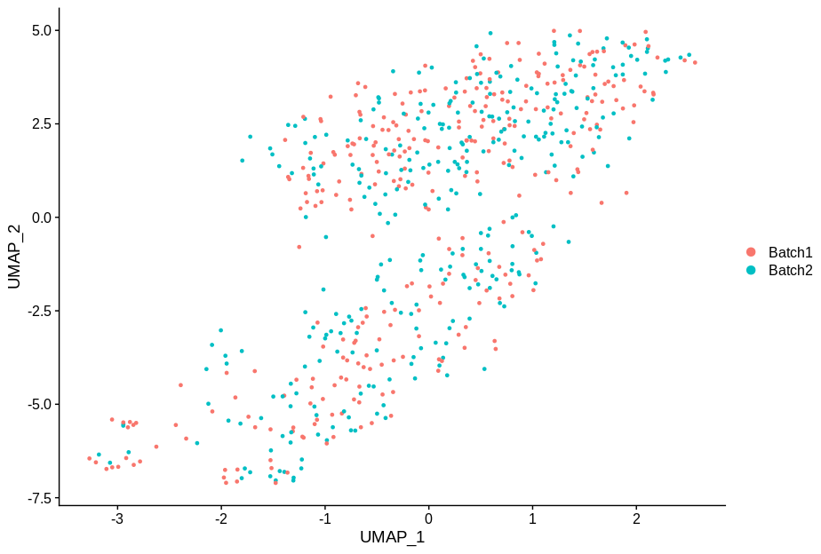
In my opinion the correct answer is that we don’t have enough information to tell if there is a batch effect here. To decide, we really need some idea of what cell type/state each cluster represents. Let’s consider two possible annotations. Here is annotation A:

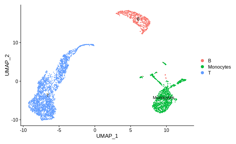
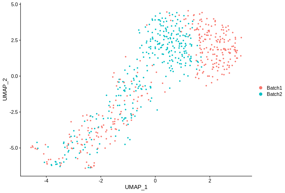
Here the sample specific clusters represent distinct cell types, Monocytes and T cells, while the reasonably well mixed cluster represents B cells. Obviously we’d want to investigate how and why there are no monocytes in sample 1 and no T cells in sample 2. But we certainly don’t want to try and use batch correction to make the monocytes look like T cells. In practice, any sensible single cell batch correction method would not try and merge these clusters and keep them far apart. Now let’s look at annotation B:

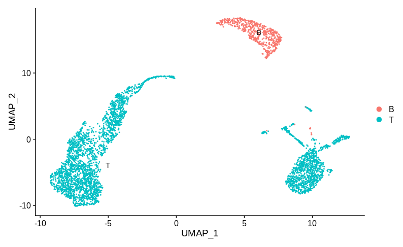
Here the T cells are split into two groups, each specific to one sample. I think most people would then be happy to claim that this is good evidence of a batch effect and try and apply a correction. Personally, I would still want more information before deciding that. I have one population of cells that are well mixed between batches (the B cells). While technical batch effects can be non-linear and effect different populations in different ways, I’d still want to know exactly how the two T cell populations differ.

My point is that the diagnosis of batch effects and the decision to correct them is fundamentally a biological one, not a technical one. Deciding a batch effect is present, is making the claim that the differences seen in the above plots are more than what we expect due to variation in T cell composition or biology. Or that we just do not care about this variation and are only interested in the similarities between batches.

How different are they really

One thing I find I am lacking in making these judgements is having a sense of how much variation is needed to drive a given split in UMAP/tSNE visualisations. I say this because in my experience basically all batch effects in single cell data are diagnosed by looking at how points cluster on some 2D representation of the data. Do you really know how different two groups of cells need to be to drive them to form two clusters on a UMAP plot?

I don’t have a deep enough understanding of the mathematics underlying UMAP (and graph based clustering methods like louvain) to be able to predict how much a transcriptome needs to change to appear separated on a UMAP plot. So instead I did some experimentation with 10X PBMC data. I loaded the data and processed it in Seurat as follows,

library(Seurat)

#' Seurat default analysis
#'
#' @param dat Raw filtered count matrix.
#' @param numPCs How many PCs to use.
#' @param clusteringRes Clustering parameter to use.
#' @return Seurat object.
quickCluster = function(dat,numPCs=75,clusteringRes=1.0){
  ss = CreateSeuratObject(dat)
  ss = NormalizeData(ss,verbose=FALSE)
  ss = FindVariableFeatures(ss,verbose=FALSE)
  ss = ScaleData(ss,verbose=FALSE)
  ss = RunPCA(ss,npcs=numPCs,approx=FALSE,verbose=FALSE)
  ss = FindNeighbors(ss,dims=seq(numPCs),verbose=FALSE)
  ss = FindClusters(ss,res=clusteringRes,verbose=FALSE)
  ss = RunUMAP(ss,dims=seq(numPCs),verbose=FALSE)
  return(ss)
}

#Start with PBMC data
pbmc =  Read10X('PBMC_4k/filtered_gene_bc_matrices/GRCh38/')
pbmc = quickCluster(pbmc)
DimPlot(pbmc,label=TRUE)

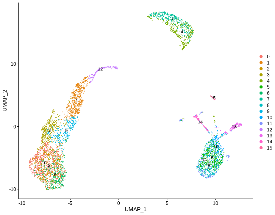
Which will look familiar from the above toy examples. I then pulled out clusters 4 and 7 as they are fairly homogeneous and used this as my base for experimentation.

w = which(pbmc@active.ident %in% c(4,7))
bb = pbmc@assays$RNA@counts[,w]
bb = quickCluster(bb)

To get at least some sense of how big a difference is needed to drive splitting of a cluster as seen by UMAP, I split this subset of cells in half and declared them my two “batches”. I then asked how many genes do I need to change to induce different visual splits in these batches. Here are the results for altering, 1, 2, 5, 10, and 20 genes.

#' Alter genes in a random subset of cells
#' 
#' @param srat Seurat object.
#' @param genes A vector of genes that will be altered.
#' @param tgtVals Values to set genes to.  Defaults to zero.
#' @param frac Fraction to modify genes for.
#' @return Altered Seurat object.
alterCellSubset = function(srat,genes,tgtVals = rep(0,length(genes)),frac=0.5){
  #Get the random subset
  w = sample(nrow(srat@meta.data),ceiling(nrow(srat@meta.data)*frac))
  mtx = srat@assays$RNA@counts
  #Alter matrix
  mtx[genes,w] = tgtVals
  #Do clustering
  srat = quickCluster(mtx)
  srat@meta.data$modified = seq(ncol(mtx)) %in% w
  srat@meta.data$batch = ifelse(srat@meta.data$modified,'Batch1','Batch2')
  return(srat)
}

gns = rownames(bb@assays$RNA@counts)[order(Matrix::rowSums(bb@assays$RNA@counts>0))]
cc1 = alterCellSubset(bb,tail(gns,1))
DimPlot(cc1,group.by='batch')
cc2 = alterCellSubset(bb,tail(gns,2))
DimPlot(cc2,group.by='batch')
cc5 = alterCellSubset(bb,tail(gns,5))
DimPlot(cc5,group.by='batch')
cc10 = alterCellSubset(bb,tail(gns,10))
DimPlot(cc10,group.by='batch')
cc20 = alterCellSubset(bb,tail(gns,20))
DimPlot(cc20,group.by='batch')

In making these plots I’ve selected the genes that are most likely to have an effect when switched off. Specifically, I have prioritised genes that are ubiquitously expressed, so turning them off will make a difference. Still, I’m shocked that in a group of cells expressing 15,000 distinct genes, changing just 5 of them is enough to introduce this large a change.

There are some vague hints of separation with just 2 genes. So instead of squinting at UMAP plots, I calculated a measure of batch mixing entropy and plotted that as a function of genes changed,

#' Calculates the batch mixing entropy for a Seurat object with meta.data 'batch'
#'
#' @param srat Seurat object.  Must have NN calculated and columns "modified" and "batch" in the meta-data.
#' @return The batch entropy.
calcEntropy = function(srat){
  tgtCells = rownames(srat@meta.data)[srat@meta.data$modified]
  cNgbs = as.matrix(srat@graphs$RNA_nn[tgtCells,]>0)
  ent = 0
  batch = srat@meta.data$batch
  kk=0
  for(tgtCell in tgtCells){
    kk = kk + 1
    lCnts = table(batch[which(cNgbs[kk,])])
    lFreq = lCnts/sum(lCnts)
    ent = ent -sum(lFreq*log(lFreq))
  }
  return(ent)
}

#Make plot of entropy by killed gene
nDropped = seq(0,20)
ents = lapply(nDropped,function(e) calcEntropy(alterCellSubset(bb,tail(gns,e))))
plot(nDropped,unlist(ents),
  type='l',
  frame.plot=FALSE,
  xlab='# Genes removed',
  ylab='Batch entropy'
  )

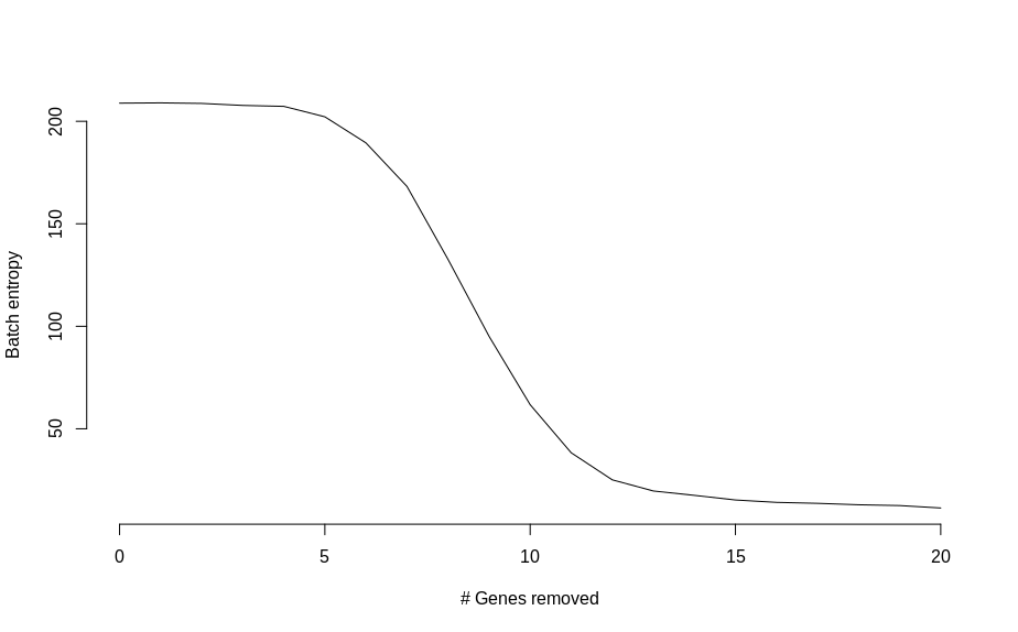
Which shows an almost monotonic trend towards lower entropy (less mixing between batches), as the number of modified genes is increased. Once the two groups of cells are basically completely separated, the change in entropy slows down.

In retrospect I guess I shouldn’t be surprised by this result. The whole point of using complex dimension reduction techniques such as UMAP is that they should be able to detect small differences. This is not a failing of UMAP, it’s doing what it should. But all it can really tell us is that there is a difference between these groups of cells. It is up to us to look at them in detail and decide if those differences are meaningful or not.

So what should we be doing? I hope to write a second post addressing this soon. But at a minimum I think we should recognise that the diagnosis of batch effects and the decision to correct for them is a biologically motivated one. The diagnosis of batch effects are made based on dimension reduction plots, which can be driven by changes in a small number of genes. Given this, is it not worth spending the time to find out which genes make batch separated clusters different (this needn’t take long)? Doing so can reveal the nature of the technical effect driving the separation or perhaps uncover interesting biological variation that would otherwise be missed.