Trying to find which genes are “different” between different conditions is probably the first thing anyone wants to do with a bulk RNA-seq experiment. When we say “different”, what is really meant is which genes show a greater difference in expression than is expected by random statistical fluctuation. The size of this change is usually expressed as a log fold change of normalised expression values between conditions and the statistical fluctuations are parameterised with a negative binomial distribution. The tools for doing this with bulk RNA-seq, such as edgeR or DESeq2, are extremely robust and mature.
So when single cell RNA-seq came along as a “thing”, it made sense to apply the same ideas to the new context. There have of course also been many attempts to use different statistical distributions and assumptions to suit the properties of single cell data better. A quick google reveals there are enough competing approaches to warrant at least one benchmarking paper.
One thing I think is overlooked in the rush to do differential expression for single cell “better” is that the biological question being asked is subtly different. Or rather, the results we as scientists most care about are not those highlighted by the traditional approach motivated by the tools developed for bulk data.
A differentially expressed gene in a bulk RNA-seq experiment represents a shift in the total expression level in a large aggregate of cells between conditions. So a doubling in expression between conditions is important and meaningful because it tells me that roughly twice as many cells are expressing gene A in one condition than the other. For single cell “differential expression” testing, most of the time what I really want to know is which genes are expressed in one group of cells and nowhere else.
Suppose I’m comparing tumour cells with the surrounding normal tissue. It’s sort of vaguely interesting to know that a gene A has roughly 3 copies in each tumour cell and roughly 1 in the surrounding endothelial cells. But you can’t target a drug, or validate well with immunohistochemistry or smFISH to “more highly expressed”. What I really want to find are the genes like CA9 that are expressed in renal cell carcinoma cells and nowhere else.
To illustrate this, I downloaded the 10X PBMC data which has an annotation and tSNE coordinates included with SoupX.
library(Matrix)
#Load PBMC data and make barcodes consistent with SoupX annotation
dat = readMM('filtered_gene_bc_matrices/GRCh38/matrix.mtx')
rownames(dat) = read.table('filtered_gene_bc_matrices/GRCh38/genes.tsv',sep='\t',header=FALSE)$V2
colnames(dat) = read.table('filtered_gene_bc_matrices/GRCh38/barcodes.tsv',sep='\t',header=FALSE)$V1
colnames(dat) =  gsub('-1','',colnames(dat))
#Load tSNE co-ordinates and clustering recorded in SoupX
library(SoupX)
data(PBMC_DR)
The B-cells are clusters 4 and 7. Let’s use edgeR to find genes that are DE compared to the rest of the cells. This is basically just the quick start edgeR analysis, but we set prior.df=0 because we have heaps of information to calculate the over-dispersion without sharing information between genes.
library(edgeR)
dge = DGEList(as.matrix(dat),group=ifelse(PBMC_DR$Cluster %in% c(4,7),'B','Other'))
mm = model.matrix(~group,data=dge$samples)
dge = estimateDisp(dge,mm,prior.df=0)
fit = glmQLFit(dge,mm)
fit = glmQLFTest(fit,coef=2)
tt = topTags(fit,n=20)
print(tt)
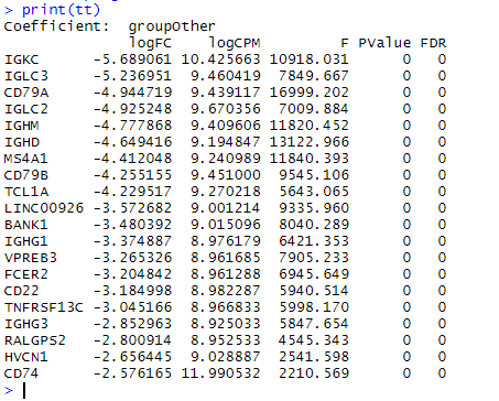
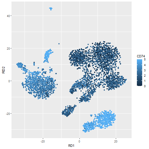
Looking at this list, it seems like my complaint is really just nitpicking. Most of these genes are recognised as being very specific to B cells and would work as good markers. I probably should have chosen a less distinct cell type to make this point. The one gene that does somewhat illustrate my point is CD74. If we plot the pattern of CD74 expression we see that while CD74 is highest in B cells (bottom right), it’s pretty ubiquitous generally. These are the sorts of genes that while genuinely differentially expressed, are not necessarily very interesting.
normDat = log(1+1e4*t(t(dat)/colSums(dat)))
dd = PBMC_DR
dd$CD74 = normDat['CD74',]
library(ggplot2)
ggplot(dd,aes(RD1,RD2)) +
  geom_point(aes(colour=ifelse(CD74>5,5,CD74))) +
  labs(colour='CD74')
Is this just nitpicking though? The list of top genes found by edgeR is really pretty good and it’s easy enough to find and filter out those that are not useful in the above way if that’s what you’re interested in. My motivation in writing this post is not to nitpick high quality tools like edgeR, but to point out that if like me, you are really just interested in what the most specific genes to a cluster are, other approaches may be more appropriate. The rather hacky thing that I’ve been doing for a while now is to use the natural language processing concept of tf-idf to get a sorted list of genes specific to each cluster. I have found this to work well for annotating and understanding a number of single cell data sets (such as this kidney paper) and has a few advantages.
The idea behind tf-idf is that it can be used to identify which words are most specific to one document out of a collection of documents (termed a corpus). Translated to transcriptomics, this is equivalent to identifying which genes are most specific to a cluster of cells relative to all other cells. There are some limitations to this; to work we have to make the scRNA-seq binary. But it captures the essence of what I often am most interested in when I’m doing “differential expression” on single cell data. This tf-idf approach is implemented in the quickMarkers function in the SoupX package. Running it to on the B-cells is simple,
mrks = quickMarkers(dat,ifelse(PBMC_DR$Cluster %in% c(4,7),'B','Other'),N=20)
mrks[mrks$cluster=='B',]
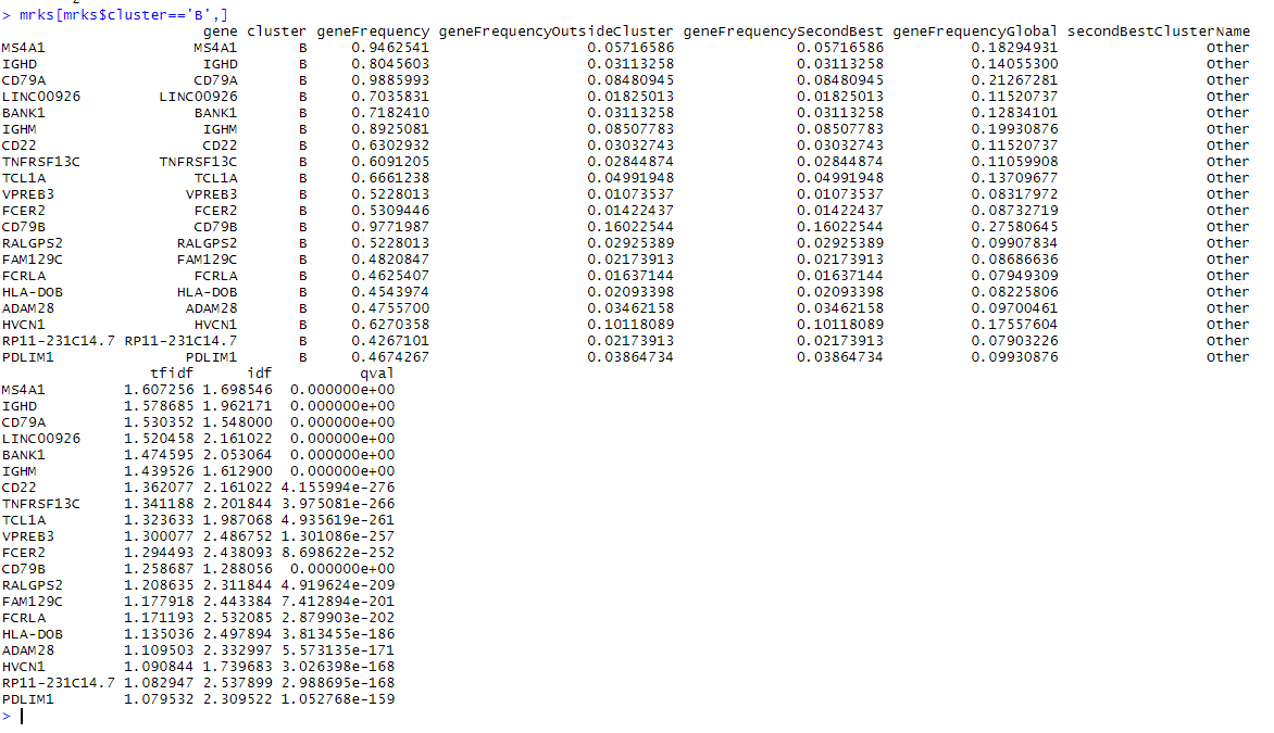
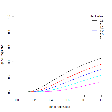
I’m struck by a few things about this. Firstly there is a lot of overlap between this list and the edgeR list, with 14 of the top 20 in common. CD74 is not in the quickMarkers list and the top gene on the quickMarkers list is ‘MS4A1’ (aka CD20), which is just about the most canonical B-Cell gene there is. I find the extra columns of meta-data very useful as well. They generally tell you about where each gene falls in the space of “what fraction of cells express it in the cluster of interest” versus “what fraction of cells outside the cluster of interest express it”. Interestingly, the tf-idf value has the property in this space that a gene with tf-idf value $t$ satisfies $\log(geneFreqGlobal) < \frac{-t}{geneFreqInClust}$. We can draw a few curves for this,
x=seq(0,1,.01)
plot(0,
  type='n',
  xlim=c(0,1),
  ylim=c(0,1),
  frame.plot=FALSE,
  xlab='geneFreqInClust',
  ylab='geneFreqGlobal')
ts = c(0.8,1,1.2,1.2,1.5,2)
cols = seq_along(ts)
for(i in seq_along(ts)){
  t=ts[i]
  lines(x,exp(-t/x),col=cols[i])
}
legend(x='topright',
  title='tf-idf value',
  legend=ts,
  lty=1,
  col=cols,
  bty='n')
There’s another dimension to this which is running time. quickMarkers runs in about 3 seconds on my machine, while running edgeR took about 30 minutes. Other marker finding methods are quicker than this, but generally fall into the “a few minutes per comparison” group rather than “basically instantaneous”. This might seem a bit trivial, but it means that I’m free to try out lots of different comparisons quickly, which can often be quite useful.
None of which is to suggest that differential expression tests as currently performed by popular packages are not useful or applicable to single cell data. But I would like to see some quantification of this property of a gene as being very specific to a cluster/cell type being considered when differential expression tests for single cell data are compared or designed. I have found it to be a useful distinction when working with single cell data and I expect others would as well.