In a previous post, I wrote about the perils of over-diagnosing batch effect. In this post I’m going to do something even more controversial and provide advice for how to deal with batch effects without using some black box “batch correction” tool. Why would you want to do this? Are batch correction tools really that bad?
It’s not that I think batch correction methods are bad. But they are opaque to varying degrees in how they change your data. So my preference is to go as far as I can, then use a batch correction method as a last resort. Resonable people may disagree, but that is my starting point.
Removing the batch effects you know
I think it’s important to recognise that “batch effects” are not some mysterious curse placed on your data. When we talk about batch effects, what we really mean are systematic differences between different parts of the experiment that we want to remove. Variability we didn’t want and obscures what we care about. Sometimes these are biological differences we don’t care about, but mostly the presumption is that the differences are driven by technical effects. Most often, this will be driven by a multitude of big and small differences, each contributing a part of the overall unwanted variability.
Perhaps we used different batches of reagents for different samples. Or used kits with different chemistries. Or entirely different single cell sequencing platforms. Or one sample had to be kept on ice over night. Or we varied the tissue dissociation protocol. Or different samples were run on different sequencing runs. Each of these changes may introduce different changes to the resulting data.
While some of these differences will result in transcriptomic changes that are hard or even impossible to predict and reverse, others are not. So the first thing to do with a data set hampered by batch effects is to remove those effects you know are present.
I will focus on the data I am most familiar with, 10X single cell expression data.
Remove swapped barcodes
The first thing I do is to remove swapped barcodes. This is super easy with the DropletUtils package (although installing the package is a bit painful).
library(DropletUtils)

cleaned = swappedDrops('data/outs/molecule_info.h5')
Most of the time this step doesn’t do much. But I’ve had cases where data run on sequencers with patterned flow cells is massively improved by this. The introduction of dual indexing in newer 10X kits should prevent this issue, but it’s worth knowing about for existing data.
Remove ambient RNA
The second thing that I routinely do is to remove the ambient RNA contamination. This can be very important as the ambient RNA looks very similar to the average of all the cells in an experiment. This is shown in the image below, which compares the average expression of each gene in the background contamination to the average expression of all cells in an experiment.
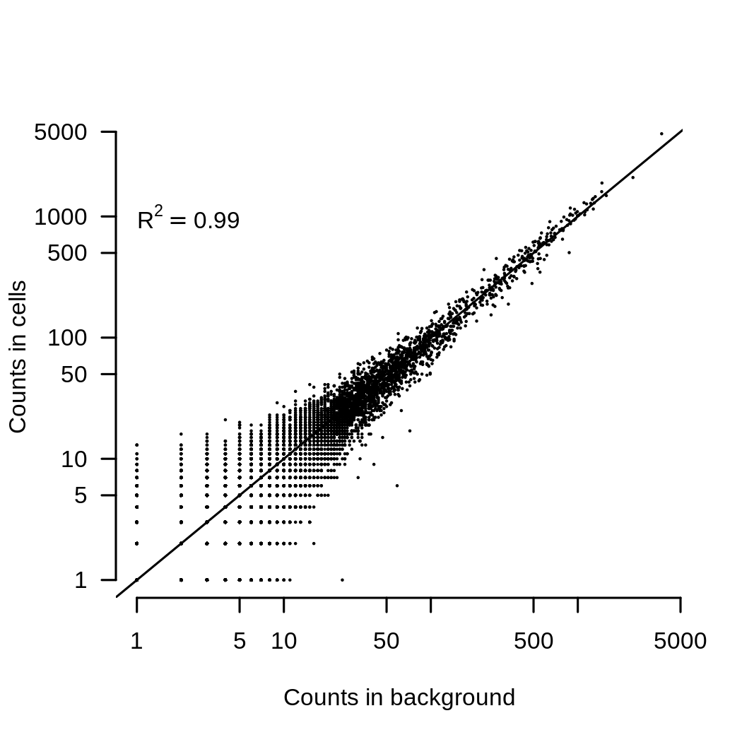
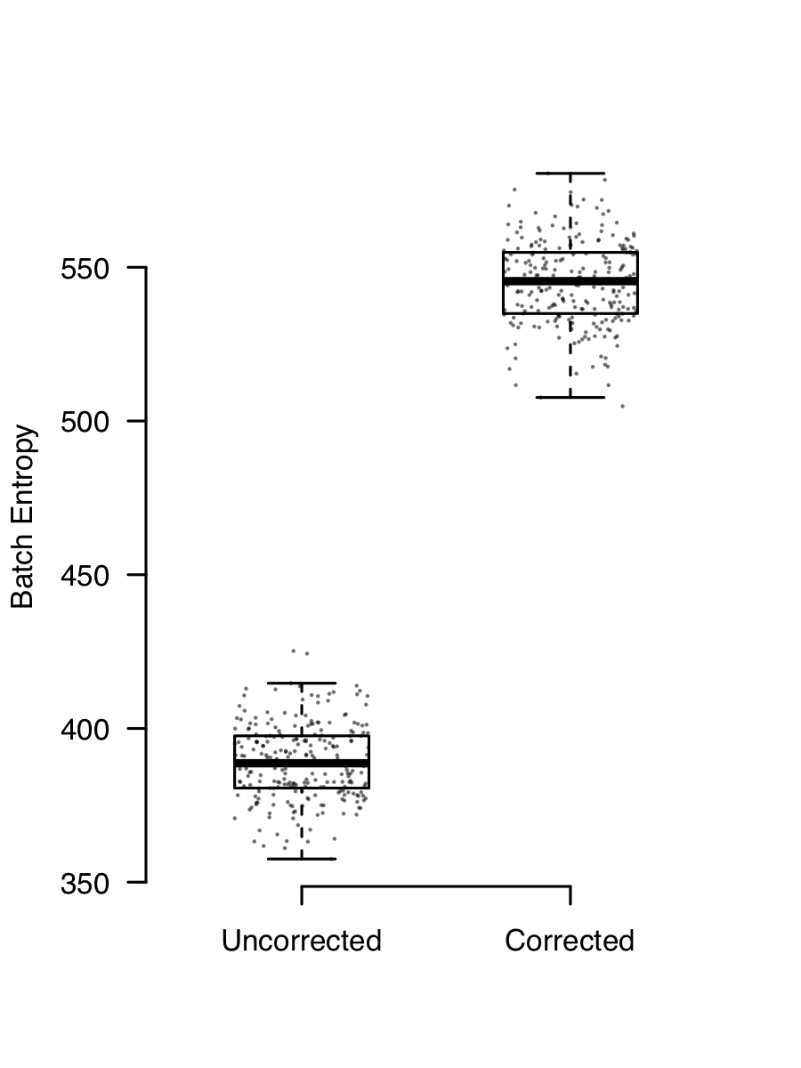
The consequence of this is that if you have two (or more) channels of data with different mixtures of cells, they will end up looking different because they have a different background added to them. Removing ambient contaimantion is easy enough. SoupX works well for me (full disclosure, I wrote it), but there are other methods too. Ambient RNA contamination creates a batch effect that is almost always present and removing it demonstrably improves integration. This plot shows the batch entropy (how well cells are mixed across channels) before and after applying SoupX to some data. The higher entropy indicates that the mixing improves when background is removed.
There’s a more complete explanation of ambient RNA contamination and its effects in the SoupX paper.
Deal with cell cycle
Having cells at different phases of the cell cycle is not strictly a batch effect. But it’s related enough and can have big effects on how data clusters, so I’m going to discuss it anyway. My main issue with cycling cells is that it can make truly unrelated cells appear related because they all happen to be in S,G2, or M phase. Most people respond to my concern with some variation of, it’s OK, I regress out cell cycle.
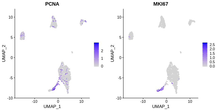
If you look at the following plot, you can clearly see that the cells in S phase (PCNA positive) and G2M phase (MKI67 phase) are distinct from whatever cluster they’re drawn from (these are papilarly cell renal cell carcinoma cells from this paper). Here I’ve used PCNA as an S phase marker and MKI67 as a marker of G2M phase as I find looking at expression of markers more reliable than Seurat’s CellCycleScoring function.
Remove cell cycle genes
But what if we drop all the cycling genes? That should make them the same as the G1 cells right? We can do this easily enough in Seurat,
phaseS = cnts['PCNA',]>0
phaseM = cnts['MKI67',]>0
altCnts = cnts[!rownames(cnts) %in% unlist(cc.genes.updated.2019),]
#Usual stuff...
altCnts@meta.data$Phase = ifelse(phaseS,'S',ifelse(phaseM,'G2M','G1'))
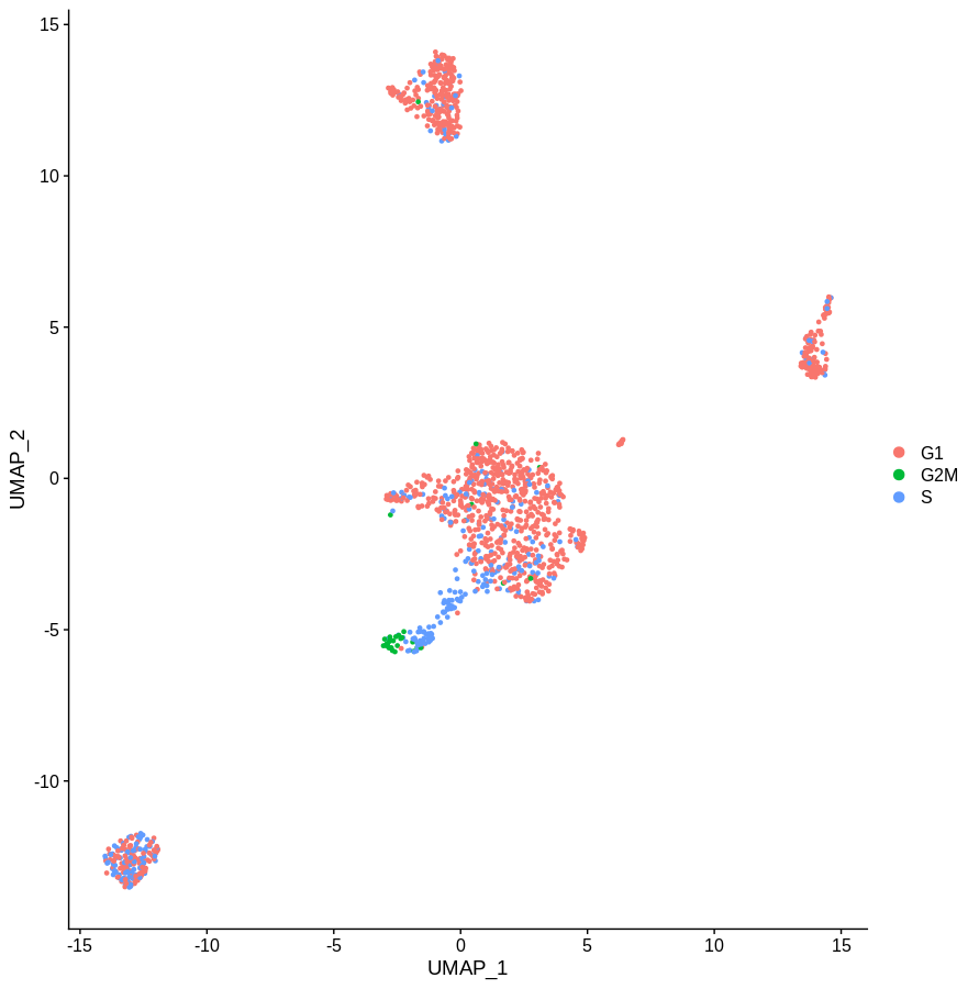
DimPlot(altCnts,group.by='Phase')
Which gives us the following plot. Obviously the definition of phase is a bit rough, but the idea is pretty clear. Getting rid of the main cell cycle genes didn’t do much. If you sourced a more complete list of cell cycle associated genes, I’m sure you’d do a better job. But given how often genes have multiple functinos in different contexts I have my doubts you’d ever get this approach to work.
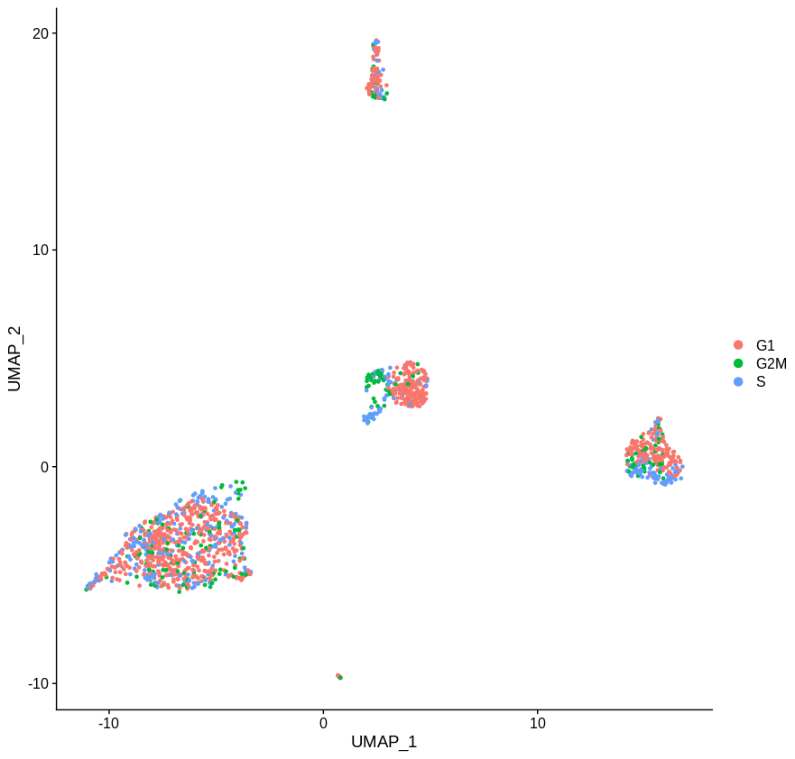
Regress out cell cycle
Very well, what if we regress cell cycle out instead. We’ll follow the Seurat vignette
reg = CreateSeuratObject(cnts)
reg = NormalizeData(reg)
reg = CellCycleScoring(reg,s.features=cc.genes.updated.2019$s.genes,g2m.features=cc.genes.updated.2019$g2m.genes)
reg = ScaleData(reg,vars.to.regress=c('S.Score','G2M.Score'))
reg = FindVariableFeatures(reg)
reg = RunPCA(reg)
reg = RunUMAP(reg,dims=seq(50))
DimPlot(reg,group.by='Phase')
Which yields the following plot. This looks better, but there’s clearly still a difference. Maybe this difference is some true difference between the underlying cell state that is not cell cycle but intrinsic to the cells themselves. But unless you’re really short on cells, or have some cell type that is only present in S/G2M phase, I’m not sure why it’s worth the bother. Just throw the the cycling cells and it ceases to be an issue.
Remove uninteresting genes
In a similar vein, there are certain conditions in which throwing out “uninteresting” genes can be very heplful for combatting batch effects. For example, There are some genes that are known to vary as a result of tissue processing (e.g. heat shock genes). In which case, you’re likely to be suspicious of any clustering that is driven by these genes. So why not just exclude them? My conservative set of genes to exclude is usually mitochondrial genes and heat shock genes. But it depends on the context of the experiment.
Obviously the information in these genes can still be useful at times, the idea is just to prevent them from driving the clustering. Probably the most robust way to do this is exclude them from your input count matrix, but preserve the information as metadata. For example,
mtGenes=grep('^MT-',rownames(cnts),value=TRUE)
redCnts = cnts[!rownames(cnts) %in% mtGenes,]
mtFrac = colSums(cnts[mtGenes,])/colSums(cnts)
red = CreateSeuratObject(redCnts)
red@meta.data$mtFrac = mtFrac
This will remove the MT genes from having any effect on the analysis, but should you wish to use the information it is available as meta data. Another alternative is just to exclude them from the highly variable genes used for calculating PCs and downstream analyses. E.g.
reg@assays$RNA@var.features = setdiff(reg@assays$RNA@var.features,mtGenes)
Just live with it.
I know batch effects look ugly on a tSNE or UMAP, and you’ll probably have at least one reviewer complain about it. But it is worth thinking about what you’re trying to achieve in your analysis and if removing a batch effect by altering the data actually furthers that goal.
For instance, a common aim of single cell analysis is to define genes that are specific to particular cell types in an experiment. On the surface, it might seem like having your cell types split into multiple clusters would hamper such efforts. But all this really does is make the task of annotating your data a bit more difficult. I’ve never had a single cell analysis where I haven’t wanted to merge the annotation of two algorithmically chosen clusters.
Although I don’t have any hard proof, I suspect that marker finding methods will do as good a job or better if you supply data unchanged by batch correction algorithms than on altered data. Certainly if you frame marker finding as a differential expression task (which I don’t think you should), you’ll get better results using methods such as edgeR or DESeq2, which require raw counts as inputs.
Conclusions
Sometimes you will have data with masses of technical variation, which won’t disappear even after doing all of the above. Or perhaps your primary interest is in looking for continuous changes in expression between cells (e.g. pseudotime). In these circumstances you have little choice but touse automated batch correction tools. But hopefully this will give you some complimentary things to try, rather than running batch correction by default.