Linear regression is one of those things that is easy to use in practice, but difficult to develop a good intuition for. At least I struggle to have a good sense of what the regression coefficients are going to look like for all but the most trivial cases.
So here is a bit of exploration of the basics of linear regression, using examples and some basic derivations of formulas. The aim being to try and develop some intuition about how linear regression behaves in more complex cases and how to interpret the coefficients in real world situations.
Simple regression
Let’s start with simple regression. That is, we have a collection of $N$ observations, where we denote the $i$th observation $y_i$. We want to do the simplest possible thing, which is explain the data with one number, which we’ll call $c$. That is, we want to fit the model
\[y = c\]This is stupidly simple and basically useless, but is instructive for being clear on how we determine what the coefficients in linear regression are.
Mathematical aside
What we really mean when we say “fit a linear model” is that we are assuming our $y_i$ are drawn from a normal distribution, with fixed variance and mean given by the right hand side of the equation above (i.e., $c$). That is, the probability (or likelihood) of the $i$th bit of data ($y_i$) in our super basic linear model is
\[l(y_i) = \frac{1}{\sqrt{2 \pi \sigma^2}} e^{- \frac{1}{2} \left( \frac{y_i- c}{\sigma} \right)^2}\]which means the probability of all our observations is
\[l(y) = \Pi_i \frac{1}{\sqrt{2 \pi \sigma^2}} e^{- \frac{1}{2} \left( \frac{y_i- c}{\sigma} \right)^2}\]So the whole trick is to pick the value of $c$ that makes the total probability of all our observations as high as possible (maximise $l(y)$). This is mathematically equivalent to minimising $-\log{l(y)}$, the negative log-likelihood, which is
\[-\log{l(y)} = \frac{1}{2}\log{(2\pi\sigma^2)} + \frac{1}{2\sigma^2} \sum_i (y_i -c)^2\]the only bit of the above which changes as we alter our linear model coefficient $c$ is the sum, so the version of our model which maximises the probability of our observations is the one that minimises
\[\sum_i (y_i - c)^2\]which is where ordinary least squares minimisation comes from. To find the minimum we do the usual thing and find where all the partial derivatives are zero. In our case, there’s just one.
\[0 = \frac{d}{dc}(-\log{l}) = 2 \sum_i c (y_i - c) \\ 0 = \sum_i (y_i -c) \\ c = \frac{1}{N} \sum_i y_i\]Intercept only
So if we fit a linear model with just an intercept, what we get is the intercept set to the mean of $y$. You probably don’t need much convincing, but let’s simulate and fit this model in R anyway. In R, the linear model language includes an intercept by default, so we fit this model with
y = rnorm(100)
fit = lm(y ~ 1)
summary(fit)
message(sprintf("The mean of y is %g",mean(y)))
which returns
Call:
lm(formula = y ~ 1)

Residuals:
     Min       1Q   Median       3Q      Max
-1.82823 -0.63107 -0.00299  0.63074  2.25832

Coefficients:
            Estimate Std. Error t value Pr(>|t|)
(Intercept) -0.04296    0.09081  -0.473    0.637

Residual standard error: 0.9081 on 99 degrees of freedom

The mean of y is -0.0429569
So the best fit value of $c$ is indeed the average of $y$ as we would expect.
One variable only
The slightly less useless version is of course where we have another variable $x$ related to $y$ in some way. If we then modify our model to be
\[y = \beta_x x\]Or we could keep a constant term (known as an intecept) and then the model would be
\[y = \beta_x x + c\]Remember what we mean by this is find the value of $\beta_x$ (or $\beta_x$ and $c$) that makes the observed $y_i$s the most probable (or likely) if the data is drawn from a normal distribution with mean $\beta_x x_i$ (or $\beta_x x_i + c$). That is, we want to find $\beta_x$ (or $\beta_x$ and $c$) that minimises
\[l(y_i) = \frac{1}{\sqrt{2 \pi \sigma^2}} e^{- \frac{1}{2} \left( \frac{y_i- \beta_x x_i}{\sigma} \right)^2} \\ \text{or} \\ l(y_i) = \frac{1}{\sqrt{2 \pi \sigma^2}} e^{- \frac{1}{2} \left( \frac{y_i- \beta_x x_i - c}{\sigma} \right)^2}\]which is mathematically equivalent to minimising (see aside above)
\[\sum_i (y_i - \beta_x x_i)^2\\ \text{or}\\ \sum_i (y_i - \beta_x x_i - c)^2\]This is a lot of formulas and not a lot of intuition. So let’s consider some made up data,
x = rnorm(1000)
y = rnorm(1000)
#Make random data with no correlation
for(i in seq(10000)){
  tmp = rnorm(1000)
  if(abs(cor(tmp,x)) < abs(cor(y,x)))
    y=tmp
}
y = y +10
plot(x,y,ylim=c(0,max(y)))
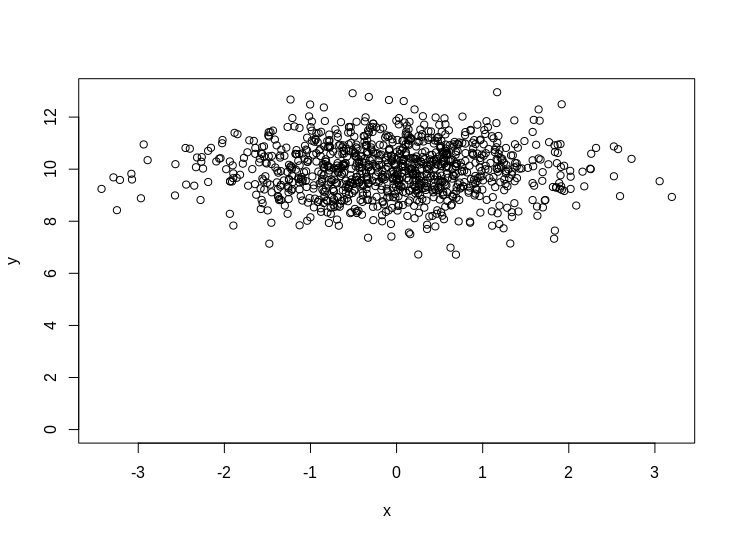
So what is your intuition as to what fitting a model with/without the intercept should look like on this data? It should hopefully be obvious that the intercept model should have $\beta_x =0$ and $c=10$. But what about the no intercept version?
fit = lm(y ~ x + 0)
summary(fit)
which gives
Call:
lm(formula = y ~ x + 0)

Residuals:
   Min     1Q Median     3Q    Max
 6.973  9.304 10.002 10.688 13.296

Coefficients:
  Estimate Std. Error t value Pr(>|t|)
x   0.2507     0.3194   0.785    0.433

Residual standard error: 10.05 on 999 degrees of freedom
Multiple R-squared:  0.0006164,	Adjusted R-squared:  -0.0003839
F-statistic: 0.6162 on 1 and 999 DF,  p-value: 0.4326
So without the intercept term, a linear model will use what it can to explain the data, and imply a relationship with the variables in the model (in this case $x$). Looking at some more formulas is helpful here. It is easy to show that the value of $\beta_x$ that minimises the probability of the data in the no intercept model is
\[\beta_x = \frac{\sum_i y_i x_i}{\sum_i x_i x_i}\]while for the intercept model it is
\[\beta_x = \frac{\sum_i (y_i - <y>)(x_i - <x>)}{\sum_i (x_i - <x>)(x_i - <x>)}\]where $<>$ denotes the mean of a variable. So the effect of including the intercept is to make the best fit for $\beta_x$ centred around 0. If you look up the definition of covariance and correlation, you’ll see that we can write the best fit value for the intercept model as,
\[\beta_x = \frac{\text{cov}(x,y)}{\text{cov}(x,x)} = \rho_{x,y} \frac{\sigma_y}{\sigma_x}\]where $\rho_{x,y}$ is the correlation between $x$ and $y$ and $\sigma$ is the standard deviation.
Which is a lot of words to arrive at a pretty basic conclusion, that in simple linear regression (with an intercept) the slope coefficient is just the correlation coefficient between $x$ and $y$, scaled by the ratio of the standard deviations.
Multiple regression
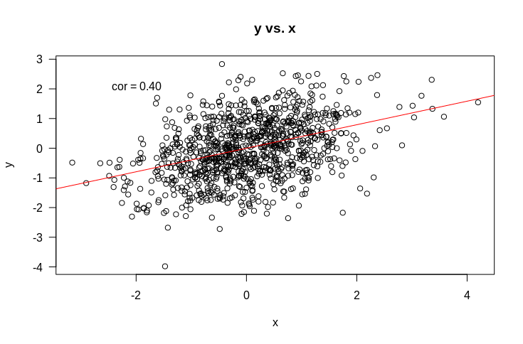
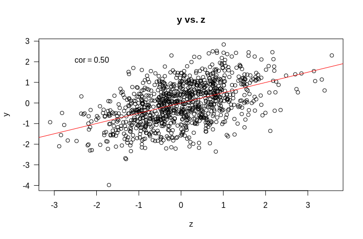
But what about the more complicated (and more interesting) case of multiple regression. That is, where we have multiple variables that we suspect might be related to $y$. Let’s start with an example. Suppose we have $y$ as before, and two variables it might be related to: $x$ and $z$. Let’s start by looking at some plots of how $y$ is related to $x$ and $z$.
So if we fit a linear model $y \sim x + z$, what would you expect the coefficients to be? Remember that the intercept term is included by default and that what this means is that we are assuming each data point $y_i$ is drawn from a normal distribution with mean $\beta_x x_i + \beta_z z_i + c$. When we fit the model, we find the values of $\beta_x$, $\beta_z$, and $c$ that make the observed $y_i$ the most probable.
It should be fairly obvious that we should expect that $c$ should be approximately 0. Suppose also that all variances are 1. If we naively extrapolate from simple regression, we might expect that the coefficients should just be the correlations (as the variance is $1$ for all variables). That would lead as to predict that $\beta_x = 0.4$ and $\beta_z = 0.5$. So let’s try it out.
fit = lm(y ~ x + z)
summary(fit)
Which results in
Call:
lm(formula = y ~ x + z)

Residuals:
    Min      1Q  Median      3Q     Max
-3.0772 -0.5872 -0.0053  0.5552  2.7472

Coefficients:
             Estimate Std. Error t value Pr(>|t|)
(Intercept)  0.004161   0.027370   0.152    0.879
x           -0.011239   0.045868  -0.245    0.806
z            0.508741   0.045798  11.108   <2e-16 ***
---
Signif. codes:  0 ‘***’ 0.001 ‘**’ 0.01 ‘*’ 0.05 ‘.’ 0.1 ‘ ’ 1

Residual standard error: 0.8631 on 997 degrees of freedom
Multiple R-squared:  0.2515,	Adjusted R-squared:   0.25
F-statistic: 167.5 on 2 and 997 DF,  p-value: < 2.2e-16
If you’re not used to reading these outputs, it says the coefficient for $z$ is 0.5, the intercept is $0$ and the coefficient for $x$ is … $0$ as well. What?! So much for out intuition. I’ve hidden another part of the picture from you here, which is how $x$ and $z$ are related to each other, which is shown by the plot below
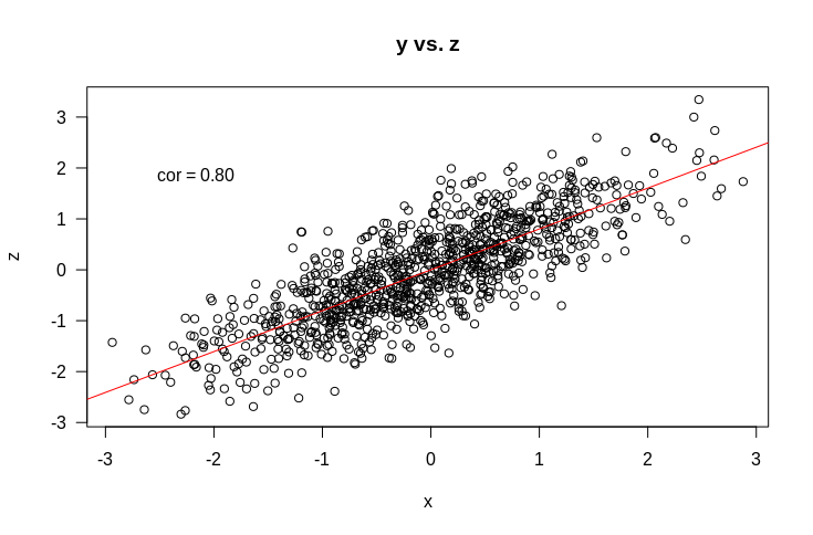
So $x$ and $z$ are correlated, which clearly feeds into the counter intuitive results above. But even when presented with all the correlations, I’d be hard pressed to intuit that the correlation between $x$ and $z$ would cause the coefficient of $z$ to be the same as if $x$ wasn’t included and $x$ to be 0. Here is the code to generate these results
library(MASS)
yx = 0.4
yz = 0.5
xz = 0.8
sig = matrix(c(1,yx,yz,yx,1,xz,yz,xz,1),nrow=3)
mat = matrix(0,nrow=3,ncol=3)
for(i in seq(10000)){
  tmp = mvrnorm(1000,rep(0,3),sig)
  cc = cov(tmp)
  if(mean(abs(cc-sig)) < mean(abs(cov(mat)-sig))){
    mat = tmp
  }
}
y = mat[,1]
x = mat[,2]
z = mat[,3]
#Make plot 1
plot(x,y,main='y vs. x',las=1)
abline(0,cor(x,y),col='red')
text(x=quantile(x,0.02),y=quantile(y,0.98),lab=sprintf('cor = %.02f',cor(x,y)))
#Make plot 2
plot(z,y,main='y vs. z',las=1)
abline(0,cor(z,y),col='red')
text(x=quantile(z,0.02),y=quantile(y,0.98),lab=sprintf('cor = %.02f',cor(z,y)))
#Make plot 3
plot(x,z,main='y vs. z',las=1)
abline(0,cor(x,z),col='red')
text(x=quantile(x,0.02),y=quantile(z,0.98),lab=sprintf('cor = %.02f',cor(x,z)))
#Fit model
fit = lm(y ~ x + z)
summary(fit)
Formulas for multiple regression coefficients
As with simple regression, we can write down exact formulas for what the best fit regression coefficients for $x$ and $z$ are. These are complicated in general, but if we make the simplifying assumption that the standard deviation of all variables ($y$, $x$, and $z$) are all $1$ these simplify massively and can be written as
\[\beta_x = \frac{\rho_{x,y}-\rho_{x,z} \rho_{z,y}}{1-\rho_{x,z}^2} \\ \beta_z = \frac{\rho_{z,y}-\rho_{x,z} \rho_{x,y}}{1-\rho_{x,z}^2} \\\]where $\rho_{a,b}$ is the correlation between $a$ and $b$. You can work through these formulas to see that I constructed the data above so that the terms would exactly cancel and conspire to make $\beta_x = 0$. In terms of building an intuition, these formulas suggest that in the mutiple regression case, the coefficients are proportional to the simple correlation between $y$ and each variable in the model ($x$ and $z$) after subtracting off some of the correlation with the other variable. As you would expect, in the case where $x$ and $z$ are completely unrelated, the multiple regression case would collapse down to what our intuition from simple regression would suggest. That is, $\beta_x = \rho_{x,y}$ and $\beta_z = \rho_{z,y}$.
So we learnt something from the one variable $y \sim x$ case, but with multiple variables we need to moderate the intuition to account for any correlation between covariates (like $x$ and $z$ in the above example).
Making things more complicated to make them simpler
Usually I tend to favour keeping things simple until you understand exactly what is happening. However, this is one case where making the situation more complex actually helps understand the simple case more easily (at least I think so). So let’s try that and extend to the case of $m$ covariates, $x_1$, $x_2$, …, $x_m$. The model we fit will than have $m$ coefficients $\beta_1$, … $\beta_m$ (plus an intercept) that we need to find. It’s pretty easy to show that the best fit values must satisfy,
\[\text{cov}(y,x_1) = \text{cov}(x_1,x_1) \beta_1 + \text{cov}(x_1,x_2) \beta_2 + ... + \text{cov}(x_1,x_m) \beta_m \\ \text{cov}(y,x_2) = \text{cov}(x_2,x_1) \beta_1 + \text{cov}(x_2,x_2) \beta_2 + ... + \text{cov}(x_2,x_m) \beta_m \\ ... \\ \text{cov}(y,x_m) = \text{cov}(x_m,x_1) \beta_1 + \text{cov}(x_m,x_2) \beta_2 + ... + \text{cov}(x_m,x_m) \beta_m\]Which is much more easily expressed in matrix notation as
\[\text{cov}(\mathbf{Y},\mathbf{X}) = \mathbf{\beta} \text{cov}(\mathbf{X},\mathbf{X})\]here $\text{cov}(X,X)$ is just the covariance matrix. To solve for $\beta$ we just invert this matrix and multiple it by the column matrix with entries $\text{cov}(y,x_i)$. If we define the entry $i,j$ of the inverse covariance matrix to be $p_{i,j}$ then $\beta_i$ is just
\[\beta_i = \sum_j \text{cov}(y,x_j) p_{i,j}\]writing out an example
\[\beta_1 = \text{cov}(y,x_1) p_{1,1} + \text{cov}(y,x_2) p_{1,2} + \text{cov}(y,x_3) p_{1,3} + ... + \text{cov}(y,x_m) p_{1,m}\]and if we take the easy case of $m=2$ (our example with $x$ and $z$ above)
\[\beta_x = \text{cov}(y,x) p_{x,x} + \text{cov}(y,z) p_{x,z} \\ \beta_z = \text{cov}(y,x) p_{x,z} + \text{cov}(y,z) p_{z,z}\]Great. This helps how?
This seems like a lot of formulas and extra complication without the promised simplification. But if we look at the above formula for a bit, we see that each of the linear regression coefficients is just the weighted sum of all the covariances between the observed data $y$ and the model variables $x_i$. So to understand the coefficients, we just need to understand what the weights, $p_{i,j}$ are.
These do have a special meaning, which is that the inverse covariance matrix (the $p_{i,j}$) are the partial correlations between $x_i$ and $x_j$ (up to a constant). I found this discussion helpful in understanding what partial correlations are. The partial correlation is basically the correlation that is left, once all the other correlations have been taken into account. The correlation between residuals rather than the variables themselves.
Visualising the relationships
Which gives us a rough idea of how to expect regression coefficients to behave. But given the results so directly depend on the various covariance matricies and their inverse, I think the best way to understand them is to visualise them.
Here’s a function to visualise the matricies inovlved. It should work as long as ComplexHeatmap is installed, which it should be as it’s great.
library(ComplexHeatmap)
visLinReg = function(data,covars,toPlot=c('cov_yx','cov_xx','invCov')){
  #Construct inverse correlation matrix
  covMat = cov(do.call(cbind,covars))
  invCov = solve(covMat)
  #And correlation with data
  corMat = lapply(covars,cov,y=data)
  corMat = do.call(rbind,corMat)
  #So beta is then easy
  beta = invCov %*% corMat
  #And this is the matrix whose rowsums give beta
  mat = t(t(invCov) * as.numeric(corMat))
  #And make a nice visualisation of this...
  library(ComplexHeatmap)
  colnames(corMat) = 'y'
  #Function to add text to cells
  text_fun_fun = function(mat,j, i, x, y, width, height, fill) {
    text_fun = function(j, i, x, y, width, height, fill) {
      grid.text(sprintf('%.02f',pindex(mat,i,j)),x,y,gp=gpar(fontsize=10))
      }
      return(text_fun)
  }
  #A less aggressive colour scheme
  cmap = c('#b2182b','#ef8a62','#fddbc7','#f7f7f7','#d1e5f0','#67a9cf','#2166ac')
  cr = circlize::colorRamp2
  #Scale inverse covariance matrix by determinate for easier interpretation
  #invCov = det(covMat)*invCov
  #cmap =circlize::colorRamp2(seq(-maxVal,maxVal,length.out=7),c('#b2182b','#ef8a62','#fddbc7','#f7f7f7','#d1e5f0','#67a9cf','#2166ac'))
  hm = list(
    cov_yx = Heatmap(corMat,
      width = unit(0.5,'npc'),
      col = cr(seq(-1,1,length.out=length(cmap)),cmap),
      layer_fun = text_fun_fun(corMat),
      column_title = 'cov(y,x)',
      cluster_rows = FALSE,
      cluster_columns = FALSE,
      show_heatmap_legend = FALSE,
      column_names_side='top',
      row_names_side='left'),
    cov_xx = Heatmap(covMat,
      col = cr(seq(-1,1,length.out=length(cmap)),cmap),
      layer_fun = text_fun_fun(covMat),
      column_title = 'cov(x,x)',
      cluster_rows = FALSE,
      cluster_columns = FALSE,
      show_heatmap_legend = FALSE,
      column_names_side='top',
      row_names_side='left'),
    invCov = Heatmap(invCov,
      col = cr(seq(-max(abs(invCov)),max(abs(invCov)),length.out=length(cmap)),cmap),
      layer_fun = text_fun_fun(invCov),
      column_title = 'inv(cov(x,x))',
      cluster_rows = FALSE,
      cluster_columns = FALSE,
      show_heatmap_legend = FALSE,
      column_names_side='top',
      row_names_side='left'),
    results = Heatmap(mat,
      col = cr(seq(-max(abs(mat)),max(abs(mat)),length.out=length(cmap)),cmap),
      layer_fun = text_fun_fun(mat),
      column_title = 'inv(cov(x,x)) * cov(y,x)',
      cluster_rows = FALSE,
      cluster_columns = FALSE,
      show_heatmap_legend = FALSE,
      column_names_side='top',
      row_names_side='left'),
    beta = Heatmap(beta,
      col = cr(seq(-max(abs(beta)),max(abs(beta)),length.out=length(cmap)),cmap),
      layer_fun = text_fun_fun(beta),
      column_title = 'beta',
      show_heatmap_legend = FALSE,
      cluster_rows = FALSE,
      cluster_columns = FALSE))
  hm = hm[c(toPlot,'results','beta')]
  tmp = hm[[1]]
  if(length(hm)>1)
    for(i in seq(2,length(hm)))
      tmp = tmp + hm[[i]]
  return(tmp)
}
There are lots of matricies we could visualise, but let’s just focus on the one that determines the $\beta$ coefficients the most directly. That is, the inverse covariance matrix times the covariance of $y$ with each $x$.
visLinReg(y,list(x=x,z=z),c())
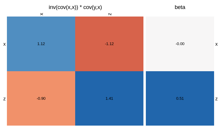
In this plot, the sum of the rows of the square matrix gives you the value of the beta coefficients. That is, each entry is the inverse covariance matrix, weighted by the correlation between $y$ and $x$ or $z$. We see that the reason $\beta_x = 0$ is that the correlation between $y$ and $x$ (top left square) is cancelled by the correction due to the correlation between $x$ and $z$ (top right square). For $\beta_z$, the correlation between $y$ and $z$ (bottom right) outweighs the correction term (bottom left). If you omit the third arguement, the function will give you a visualisation of all the matricies involved.
visLinReg(y,list(x=x,z=z))
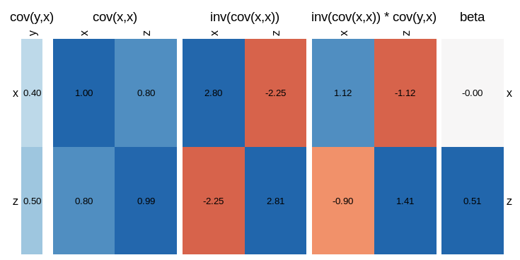
Which gives a much more complete overview of all the relationships involved.
I’m sure at this point someone will point out that there’s some inbuilt R command that does this already, but I found this useful in developing my understanding of what multiple linear regression is doing. As a final example, let’s simulate a much more complicated situation with $6$ covariates.
#Make up a correlation struture
nVar=6
ss = matrix(rnorm((nVar+1)**2,sd=1),nrow=nVar+1,ncol=nVar+1)
#Make it positive-definite
ss = ss %*% t(ss)
#Make data
dat = mvrnorm(1000,mu=rep(0,nVar+1),Sigma=ss)
y = dat[,1]
dat = dat[,-1]
dat = lapply(seq(nVar),function(e) dat[,e])
names(dat) = paste0('x',seq(nVar))
visLinReg(y,dat)
This will obviously be different every time you run it, but here is an example.
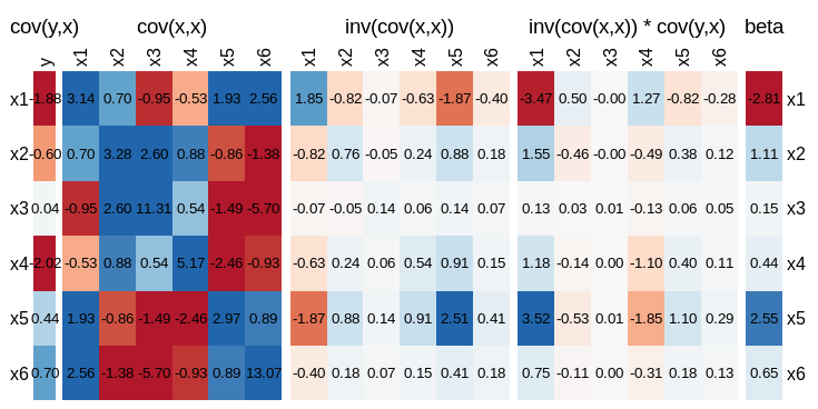
From which you can see that the coefficient of $x_5$ is driven more by the contribution from $\text{cov}(y,x_1) * \text{cov}(x_1,x_5)$ than the covariance of $y$ with $x_5$. Worse still is $\beta_4$, where the sign of the coefficient is different from what you would intuit if you just considered $\text{cov}(y,x_4)$.
Conclusion
Having gone through all that, I’m not sure I’m really all that much closer to having a reliable intuition for how to interpret linear regression coefficients. There are some simple cases, where it’s clear what the intuition is. If all covariates (the $x_i$s) are uncorrelated, the regression coefficient $\beta_i$ is closely related to the corelation between $y$ and $x_i$.
But in general, it is essential that we understand how covariates relate to one another (the covariance matrix) and their partial correlation (the inverse covariance matrix). It is easy to construct cases where the linear regression coefficient for $x_i$ is driven not by the correlation between $y$ and $x_i$, but by the relationship between $y$ and $x_j$ together with a correlation between $x_i$ and $x_j$.
I guess the upshot of all this, beyond some fairly clear intuition about how to interpret simple linear regression with one variable, is to always inspect the covariance and inverse covariance matricies. This will at least ground the interpretation of coefficients in how much connection there is between the $x_i$s. The above code will give a quick visualisation of this, but you could also just print the things in R, or I’m sure there are other functions/packages around.